Isochrones from point-layer

The openrouteservice offers an interesting endpoint that is most commonly used in reachability analyses. This is the /isochrones-endpoint that we will now have a look at. As the term isochrone is probably not too well known, let’s have a look at it first.

What is an isochrone?

An isochrone is a contour line of common time.
In GIS analyses, the common time used is usually travel time from a given point. Thus, an isochrone defines a polygon wherein all points are reachable from a given point in a given time, using a certain mode of travel

Here is a classic example for a 15-minute walking isochrone, starting at the conference venue.

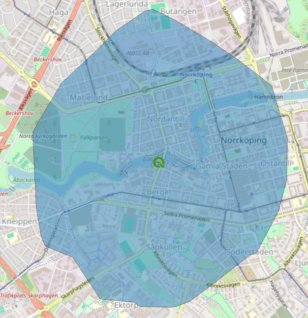
Fig. 38 15 Minute foot isochrone from Visualiseringscenter C

The resulting area, however, obviously includes points not reachable by foot:

• the Motala ström river

• the interiors of buildings not publicly accessible

• train tracks

• …and a lot more.

This showcases a central, important point about an isochrone.

The particularity of isochrones

While isochrones are usually shown as polygons, the actually reachable spots are points on the road network. In this case these which are just on the limit of being reachable in time.

These are then used to generate a polygon, creating the illusion of “this area is reachable in time”. The resulting shape is non-unique, and there is no correct shape - just less bad shapes.

As humans, we usually are able to interpret this correctly, but it is important to keep this limitation in mind.

How to calculate an isochrone?

The simplest way is the Isochrones from Point processing algorithm.

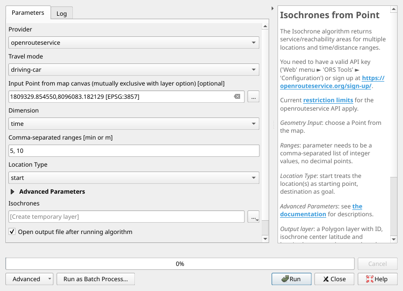
Fig. 39 Processing algorithm: Isochrones from Point

Most parameters are explained in the help text on the right side.

For us most important are:

1. Provider
   where we need to choose the one we set up earlier

2. Travel mode
   whether we go by foot, by car, …

3. Range(s)
   where we specify the travel time.

The three dots on the side of Input point from map canvas let us choose a starting point from the map canvas.

A click on Run then calculates an isochrone. This is the tool used for the calculation of the isochrone in the example above.

An isochrone-based analysis

More important for real-life analyses is the Isochrones from Point-Layer processing tool.

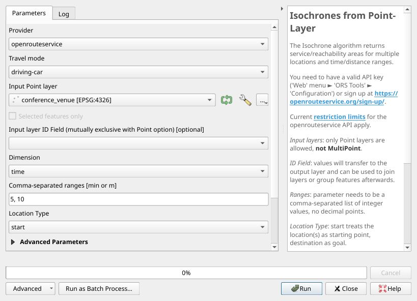
Fig. 40 The Isochrones from Point-Layer user interface

The parameters are very similar, except for the input:
Instead of inputting a single point as before, we now input a point layer, and calculate the same isochrone(s) for every point in this layer.

The analysis we want to conduct is to answer the following:

What percentage of Stockholm’s population can reach a doctor’s office by foot when sick?

As input, we will use a list of doctors in Stockholm, provided in the .gpkg-format. We will use this as an input to the algorithm, and calculate foot-walking isochrones for 650[1] metres. We use destination as our Location Type, as we want to know who can reach a doctors office, not the inverse.

Minutely limit

There is a minutely limit that we run into. The plugin will automatically retry with more and more time gaps. For bigger analyses, we will also have to respect the daily limit, but this won’t be an issue here.

Details can be found here: https://account.heigit.org/info/plans

This should result in the following:

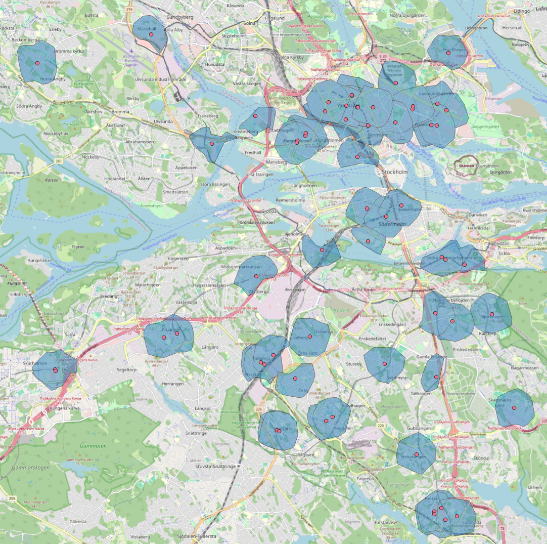
Fig. 41 650 metre foot-walking isochrones to all doctors in Stockholm, Sweden

Now that we have the areas from which the doctors offices area reachable, the remaining question is how much of the Stockholm population lives in these isochrones.

For this, we provide a Stockholm population dataset, again using .gpkg-format. This consists of a 400m radius hexagon grid over Stockholm, where every hexagon contains a population-attribute that denotes the amount of people living in this hexagon.

To not complicate the analysis too much, we select every hexagon that is in any way overlayed by one of the isochrones. This does “extend” our range by quite a bit, but not all sicknesses have the same severity, and the resulting ranges are still walkable. It does introduce some fuzziness to the analysis, but given that we are summing population on a 400 meter grid, this seems reasonable.

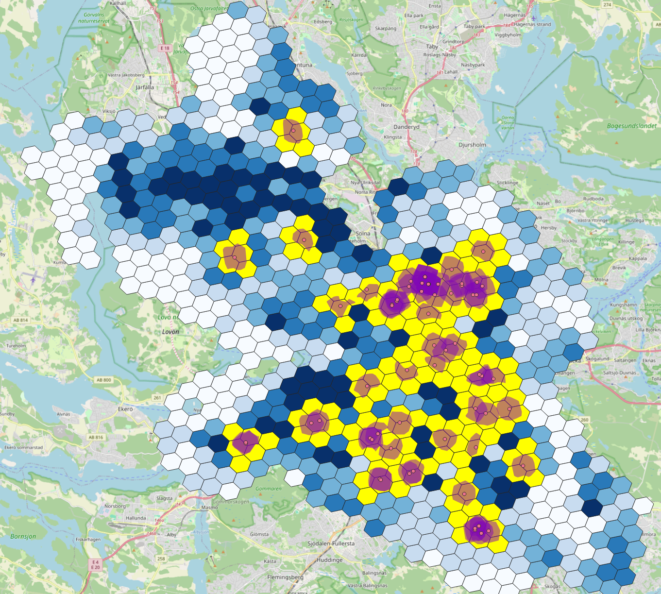
Fig. 42 Population hexagons overlapped by isochrone polygons

We can now sum up the population in those isochrones and get a sum of 544.397 people. The total population of the areas of Stockholm that are part of our analysis is 1.188.609. Thus, around 50% of the Stockholm population have “easy” foot access to a doctors office when sick.

---

[1]

This value is taken from a recent period of sickness and is the exact distance from my home to my doctor; It was barely walkable when sick.