Snapping

The /snap endpoint is used to map points anywhere on earth to the nearest point on a road network that is accessible with a given profile.

The process can be thought of as similar to geocoding. In geocoding, we translate a written address or location to a geographic coordinate. In comparison, snapping translates a given geographic coordinate into a coordinate on the road network. This is then used in routing, since routing happens on the road network.

A simple example

To get a feeling for this, we use the Snap from Point processing algorithm.

Choose a point on the map (that is not on a road) as an input, select a suitable profile and run the algorithm:

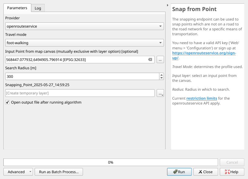
Fig. 50 The Snap from Point tool

The example here is the conference venue using foot-walking as the profile - the coordinates designate exactly the point where the “museum”-symbol for Visualiseringscenter C is.

The result is the following:

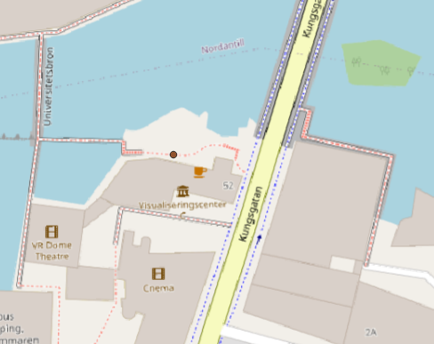
Fig. 51 The point on the road that Visualiseringscenter snaps to

This is rather expected - we will see some of the pitfalls that snapping can bring in the following section

Data (preparation)

As an example, we will look at the Heidelberg hospital landscape. The goal is to match all hospitals to the road network.

The data is available here: Point Layer: Hospitals in Heidelberg

Data preparation using the QuickOSM plugin

To get data, we use the QuickOSM-plugin and the preset of hospitals in Heidelberg

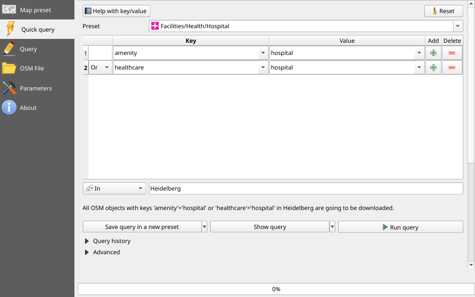
As a result, we get a point- and a polygon-layer - a bit unexpected, but given the OpenStreetMap data model this makes sense.

A hospital is usually a building, so we first need to convert the polygons into points representing the hospitals. For this, we use the same process the OSM uses to draw the red crosses representing hospitals. This is the Point on Surface algorithm, which gives us one point per polygon

We can now join this to all hospital information that are entered into the OpenStreetMap as nodes directly.

Looking at the resulting data, it turns out that a bunch of barrier, entrance or plaque nodes is also present in our data set. These are easily detected and deleted, and a lot of unnecessary fields are deleted as well.

Snapping Heidelberg hospitals

We can input our data into the Snap from Point Layer processing algorithm.

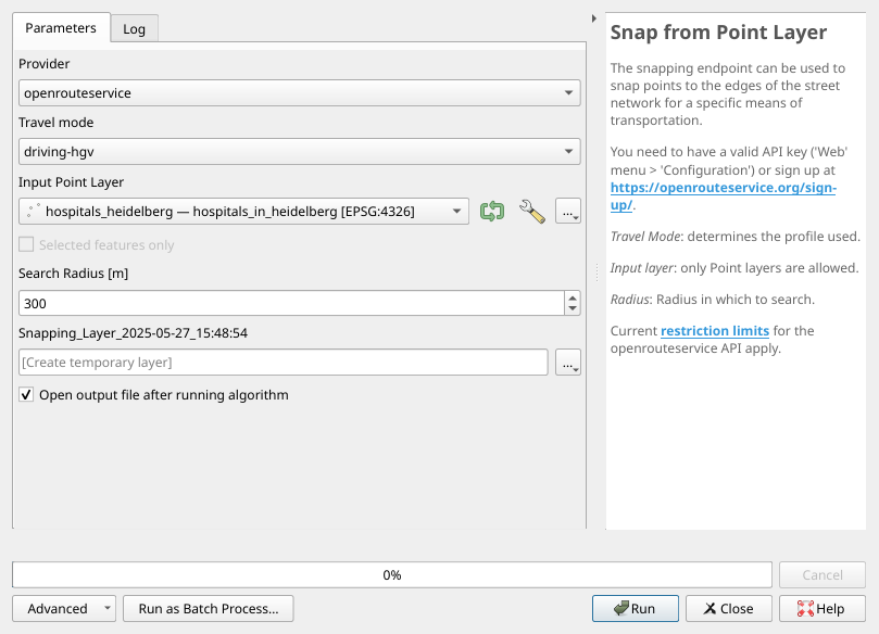
Fig. 52 The Snap from Point Layer tool

This results in the following points: The input hospitals are marked with the common red cross, the output points don’t have special styling. Colors were chosen for easier assessment of the mapping.

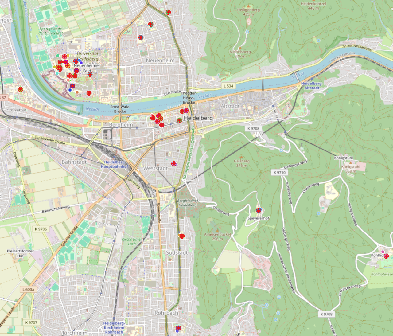
Fig. 53 Hospitals snapped to the road network

Usually, the snapped points are rather close to the input points. In the middle of Heidelberg, south of the river, almost no snapped points are visible. They mostly overlap with the input points.

However, one interesting artifact is in the northwestern part, near the river bend north of the zoo:

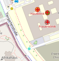
Fig. 54 Two input points snap to the same output

Here, we see three input points, yet only two output points, although we’d expect the middle hospital to snap to the middle of Tiergartenstraße.

In fact, the third snapped point is below the lower snapped point. All across the hospitals around them, results are unusual. As an example, think about why the upper hospital in the example snaps to a road near Tiergartenstraße, not to the road directly above it.

Why snapping is often counter-intuitive

First, snapping is dependent on the routing profile used. Any coordinate will only be snapped to the road network for that profile.

As an example, imagine a valley with a river inside. On one side of the river runs a street, on the other side a small footpath which a hiker can safely travel, a mountain biker might also be fine on, but is not suited for road bikes and even forbidden to travel by car.

Imagine the input coordinate to be on the river bank of the footpath, opposite of the river. Using the foot-hiking-profile will snap the input to the footpath, as will using the cycling-mountain-profile. Using the cycling-road-profile and the driving-car-profile will snap the input to the road on the other side of the river. While on first glance this might be unexpected, giving it a thought will probably clear up the confusion.

The foot-walking-profile, however, might snap to the footpath or it might not. If the footpath has an unsuitable sac-scale key, it will not be included in this profiles road network. This distinction, however, might not be reflected on the map visualizing the path - or at least not in an intuitively graspable way.

Now imagine the same situation, but the footpath is replaced by a gravel track that cars can drive on. As such, it is definitely suitable for all cycling-* or foot-* profiles. Still, this track might not be included in any road network for multiple different reasons.

Let’s say there is a barrier disallowing access to the gravel road. If this barrier is simply tagged as a node with the barrier=gate-tag, this gate might in reality be open all the time. A routing algorithm, unfortunately, does not know that - it only sees the barrier=gate node and has to assume that this forbids access, as this is the purpose of the barrier. Barring any other information, the default has to be to exclude the road from the network.

Let’s say there is no barrier, but a section of the gravel road - the one that is closest to our input - has a tracktype=*-key that is deemed unsuitable to the driving-car-profile. Maybe it was fixed only recently, and tagging hasn’t been updated. Maybe this is only the case in the winter season, but it is easier to set up in this way. Maybe the reason is not the track, but that you have to be an experienced driver to safely get there, and it has happened too often that cars needed to be rescued for that.

Whatever the reason - if the street is closer to the input than a suitable section of the gravel track, the snap will go to the road, not the track.