
Matrix#
What is a distance matrix?#
A distance matrix is a table that shows the distances or travel times between multiple locations. For every pair of locations, it provides the distance or travel time from one location to another.
We will calculate a measure called closeness using the Matrix from Layer tool. Closeness
is a concept from network analysis that reflects how near a location is to all other locations in the
network. A point with high closeness has short travel times or distances to many other points, meaning it’s well-
connected and easily reachable.
In our case, we’ll use the travel time or distance matrix to calculate the average travel cost (time or distance)
from each point to all others. Points with lower averages are considered more “central” in terms of closeness,
making them important for accessibility planning, service placement, or emergency response scenarios.
FROM_ID |
TO_ID |
DURATION_H |
DIST_KM |
|---|---|---|---|
Starbucks |
Starbucks |
0 |
0 |
Starbucks |
Urban Cup |
0.0842861 |
2.03287 |
Starbucks |
Tim Hortons |
0.184625 |
5.96267 |
Urban Cup |
Starbucks |
0.07724 |
1.89601 |
Urban Cup |
Urban Cup |
0 |
0 |
Urban Cup |
Tim Hortons |
0.162216 |
4.8294 |
Tim Hortons |
Starbucks |
0.185727 |
6.11282 |
Tim Hortons |
Urban Cup |
0.16033 |
4.73623 |
Tim Hortons |
Tim Hortons |
0 |
0 |
How to calculate a distance matrix?#
Create a grid and centroids#
Zoom in to your favourite city and set the map scale to approximately 1:5,000. Then, open the Create Grid tool from
the Processing Toolbox. Set the Grid Type to Hexagon (polygon) and specify both horizontal and vertical spacing as
500 meters.
Next, click the “Set to current map canvas extent” button to ensure the grid covers the visible area. Leave the other parameters at their default values and run the algorithm.
Once the hexagonal grid is generated, open the Centroids tool and apply it to the grid layer to create a new point
layer with the centroids of each hexagon.
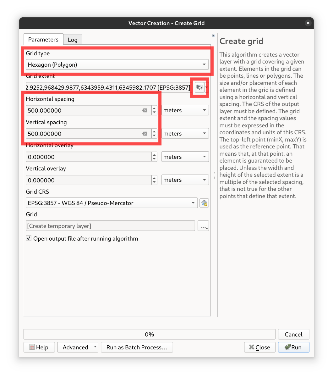
Fig. 43 The create-grid tool and the settings to be applied#
```{figure} ../_static/media/matrix/grid_map.png
---
width: 100%
alt: The created grid
---
The created grid
Run matrix from Point Layer#
With the “Matrix from Layer” tool in ORSTools, we can now calculate the distances and travel times between all centroids in the hexagonal grid. This allows for a comprehensive analysis of accessibility and connectivity across the study area.
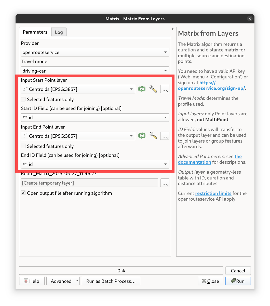
Fig. 44 The Matrix from Layer tool user interface#
Aggregate the matrix results#
Use the “Aggregate” tool from the Processing Toolbox to calculate the mean travel times and distances for each origin
point. Set the “Group by expression” parameter to FROM_ID. In the Aggregates table, delete the TO_ID
field. Then, set the aggregate function for both DURATION_H and DIST_KM to mean and for the FROM_ID to
last_value. Once everything is set up, click Run to execute the algorithm.
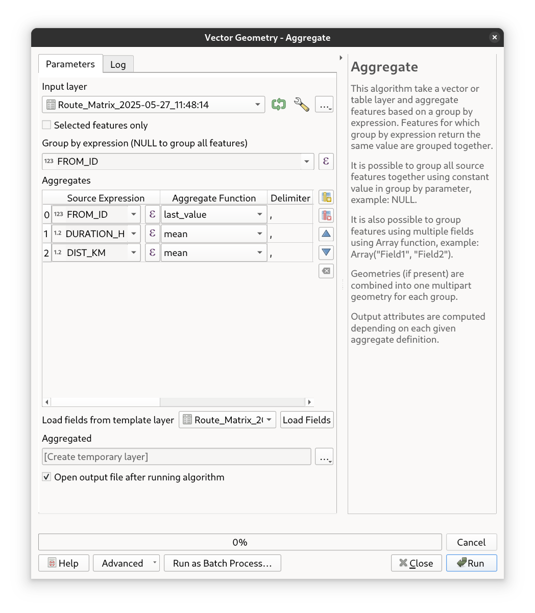
Fig. 45 The aggregate tool and the settings to be applied#
Join results back to the grid#
Open the Layer Properties of the original grid layer and navigate to the “Joins” tab. Add a new join by linking the ID
field of the grid layer with the FROM_ID field of the aggregated layer. This will attach the calculated mean travel
times and distances to each corresponding hexagon in the grid.
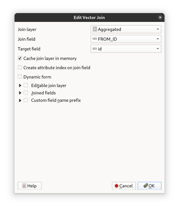
Fig. 46 The settings for the join#
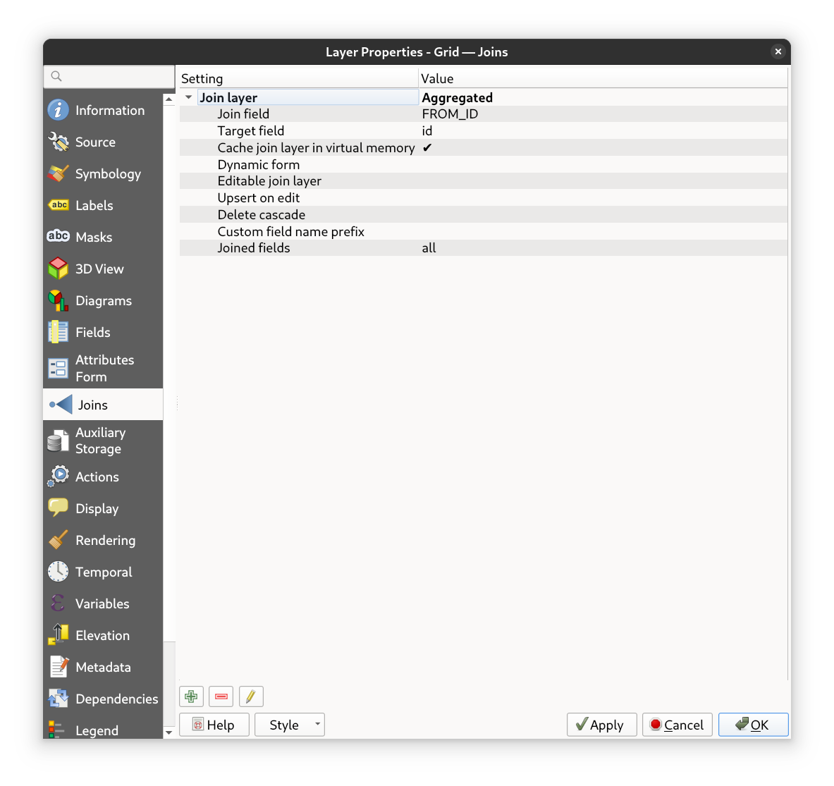
Fig. 47 The resulting join in the layer properties#
Style it!#
Next, go to the Symbology tab in the Layer Properties of the grid layer. Set the Value field to either
Aggregated_DURATION_H or Aggregated_DIST_KM, depending on what you want to visualize. Change the Symbology Type
to Graduated, choose your favourite color ramp, set the transparency of the main symbol to ~75%, and click
Classify to generate the categories. Finally, click OK to apply the style and view your results on the map.
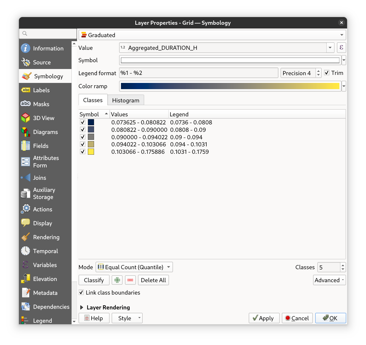
Fig. 48 The settings for the styling#
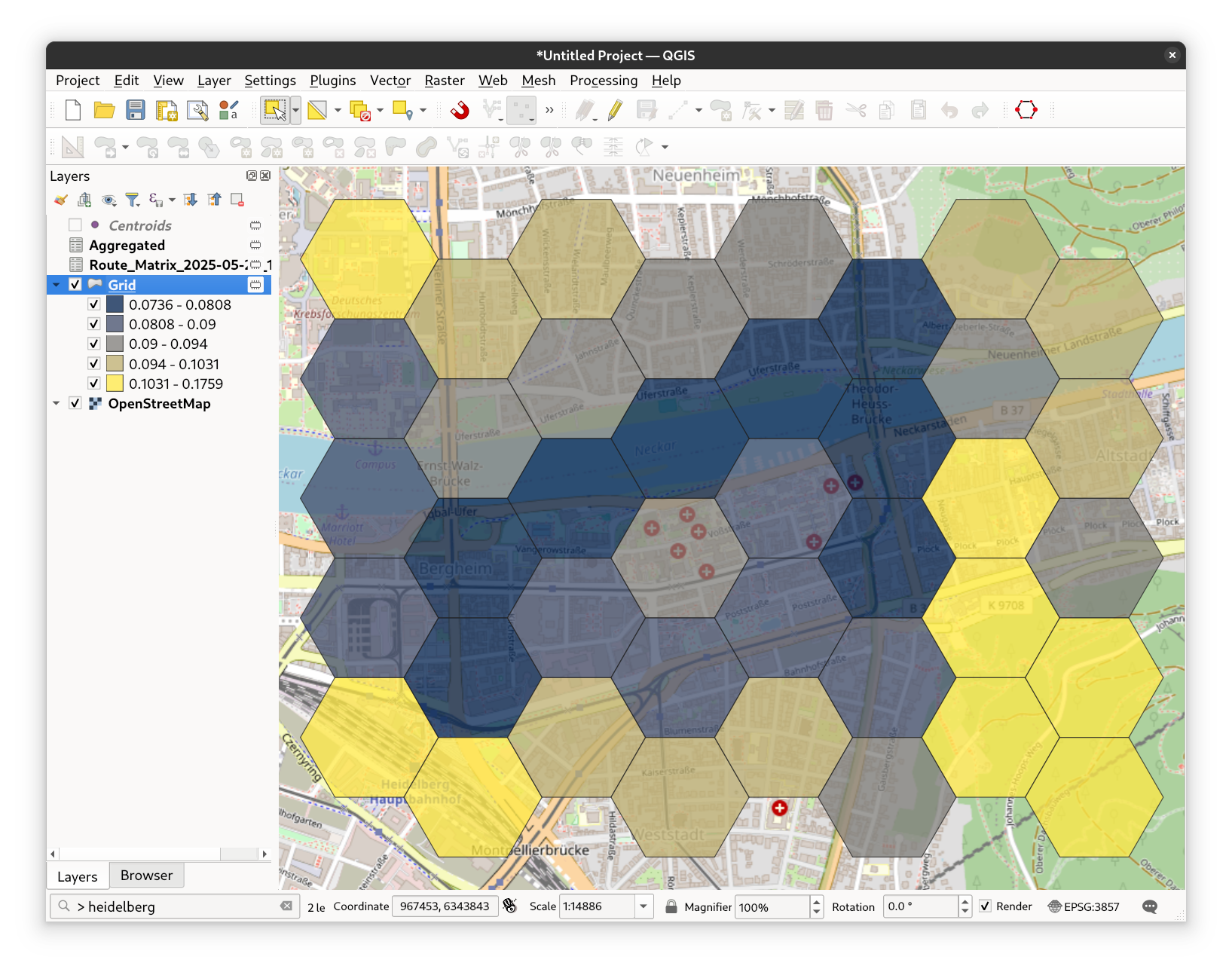
Fig. 49 The resulting styled layer#
Understand the results#
The map displays the closeness centrality of various areas based on travel times or distances. Closeness centrality is a measure that helps to assess how easily accessible a location is relative to all other locations within a network. Areas with lower closeness centrality values indicate better accessibility. These locations have shorter average travel times or distances to all other points in the network, making them more central and well-connected. Such areas are ideal for placing facilities that need to be easily reachable from many different locations.
In contrast, higher closeness centrality values point to less accessible areas. These locations tend to have longer average travel times or distances to other points, suggesting that they are more peripheral or isolated within the network. Such areas may be candidates for transportation improvements to enhance connectivity.
Closeness centrality has several practical applications. It can support decisions about where to place public services such as hospitals or fire stations, assist in urban planning and accessibility assessments, help identify regions that require better transportation links, and aid in evaluating the coverage of services across a geographic area.